


 9 / 28

Ten Year Network Development Plan 2015 Annex F |
9
P
GC
-15%
-2% for LNG
P
GC
P
GC
+15%
+2% for LNG
€
35% of the
Max. Supply
Potential
Max.
Supply
Potential
GWh/d
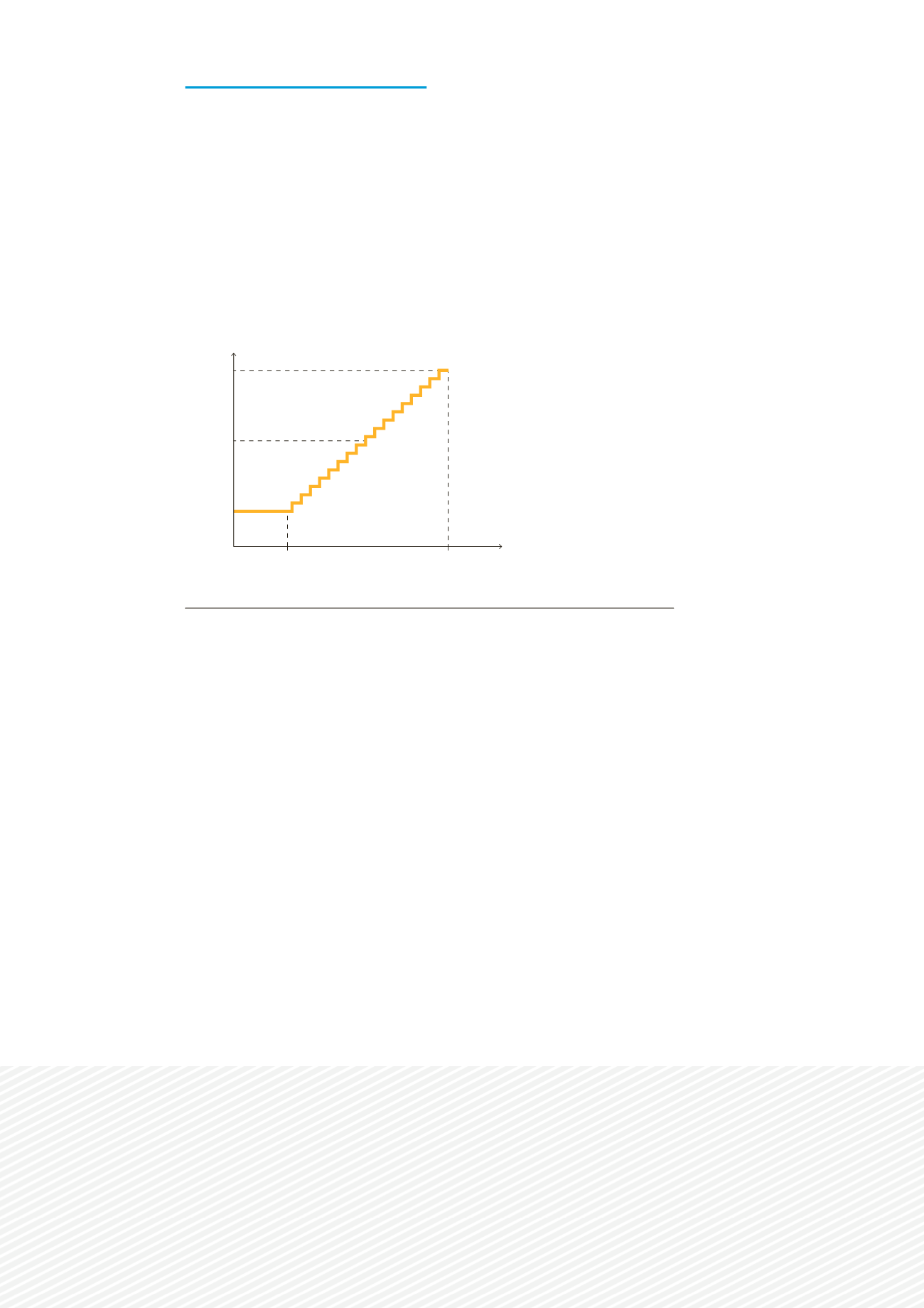
Figure 2.1:
Supply curve
2.5.3 Definition of the supply curves
Within the modelling tool, each supply source is described as a supply curve based
on the Supply Potential and Global Context scenarios. It represents the increasing
supply cost on the long run when demand is increasing (to be distinguished from
the constant price compared to volume once gas has been contracted). The curve
is built on:
\\
The yearly average import price of gas as defined in the Global Context
Scenario (P
GC
)
\\
The Supply Potential Scenarios of each source
Figure 2.1 illustrates the construction of the curve of given source on a given year:
Compared to the CBA methodology published on ENTSOG website a ± 15% range
has been used for pipe gas sources and ± 2% for LNG instead of a uniform ± 10%.
Such changes were necessary to:
\\
Ensure the necessary overlap of the curves when one source becomes
cheaper or more expensive than the other ones
\\
Reflect the small influence of Europe on the global LNG market
In addition the low point of the curve of each supply source is now based on a
constant 35% of the Maximum Supply scenario (which is the average of the ratio
between the Maximum and Minimum Potential scenario of each source). This
modification ensures a more even split of the sources in the EU gas supply mix.
A specific curve has been defined for the European indigenous production (conven-
tional, shale gas and biogas). The curve is set flat at the level of the average import
gas price as defined by the Global Context with a thirty percent discount. Such
rebate derives from the fact that the considered price information for indigenous
production is rather the production cost than the wholesale price. It enables to
include the producer surplus on EU territory within the EU social welfare assessed
by the methodology as requested by the New TEN-E Regulation.