


 138 / 258


1660
Butler-Thompson et al.:
J
ournal of
AOAC I
nternational
V
ol.
98, N
o.
6, 2015
laboratory water and discard eluent. Air-dry each cartridge by
pulling a vacuum until no more effluent is observed. Close
each stopcock. Place a 5 or 10 mL volumetric flask under each
cartridge. Add 4.4 mL 30% acetonitrile to each cartridge. Open
each stopcock and elute vitamin B
12
into the volumetric flasks.
(
4
)
Final dilution
.—For samples collected in 10 mL
volumetric flasks, dilute to volume with water. For samples
collected in 5 mL volumetric flasks, in a hood add 0.1 mL
freshly prepared 0.4% KCN to each volumetric flask. Place
prepared samples in a 95°C oven for at least 1.5 h, but for no
more than 4 h. After at least 1.5 h, remove samples from the oven
and cool to room temperature. Dilute to volume with laboratory
water. Filter an aliquot of each standard and prepared sample
through a 0.45 µm syringe filter into an autosampler vial.
(c)
HPLC analysis
.—(
1
)
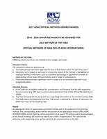
System setup and configuration.—
See
Figures
2011.10A
and
B
for configurations.
(
2
)
Instrument
operation
conditions
.—(
a
)
Run
time
.—30–35 min.
(
b
)
Injection volume
.—900 µL to 2.0 mL.
(
c
)
System configuration.—See
Table
2011.10E
.
(
d
)
Isocratic pump
.—Mobile phase D: 2.5% acetonitrile.
Flow rate: Adjust so that vitamin B
12
elutes from the size-
exclusion column between 10.5 and 14.5 min. Typical flow
rates, 1.1–1.2 mL/min.
Note
: To determine an appropriate
flow rate, connect the size-exclusion column directly to the
UV-Vis detector and inject the high standard. Adjust flow rate as
necessary so that vitamin B
12
elutes between 10.5 and 14.5 min.
(
e
)
Gradient pump
.—Mobile phase compositions: mobile
phaseA, 0.4%TEAin laboratory water, pH 5–7; mobile phase B,
0.4% TEA and 25% acetonitrile in H
2
O, pH 5–7; mobile phase
C, 0.4% TEA and 75% acetonitrile in H
2
O, pH 5–7. Determine
an appropriate gradient to elute vitamin B
12
in 23–30 min and
resolve vitamin B
12
from riboflavin using the information in
Table
2011.10F
. (
See
Figure
2011.10C
.)
(
f
)
Gradient pump flow rate
.—1.0 mL/min.
(
g
)
Detector
settings
.—Detection
wavelengths
and
bandwidth, 550 and 10 nm, respectively.
(
3
)
HPLC of standards and samples
.—Make 3–4 injections
of a working standard and verify the precision of those injections
is ≤3%. If the system is working properly, inject a set of 3–6
working standards once, a set of 1–14 samples, and another set
of 3–6 working standards. Every set of 1–14 samples should be
bracketed by standards of appropriate concentration.
F. Calculations
(a)
Chromatography
.—Visually inspect each standard and
sample chromatogram and verify that vitamin B
12
is resolved
from all other peaks in the chromatograms (Figures
2011.10D
and
E
).
(b)
Measurement of peak area
.—Peak areas are measured
with a data system. Before calculating the vitamin B
12
concentrations of samples, compare the vitamin B
12
peak areas
of the standards with the vitamin B
12
peak areas of the samples
and verify that the vitamin B
12
peak areas of the samples are
within the range of the vitamin B
12
peak areas of the standards.
(c)
Calculation of standard concentration
.—
WS = S
w
× P × A/200
where WS = working standard concentration in μg/L;
S
w
= amount of vitamin B
12
standard weighed in mg;
P = purity of USP reference standard in μg cyanocobalamin
(vitamin B
12
)/mg of the standard; A = aliquot of vitamin
B
12
intermediate standard used (0.5, 1, 2, 3, 4, or 5) in mL;
and 200 = dilution volume in mL.
(d)
Preparation of standard curves
.—(
1
) At each standard
concentration, average the peak area of the standard injected
at the beginning of a set of samples with the peak area of the
standard injected at the end of the set of samples. Prepare a
standard curve by performing linear least squares regression
Figure 2011.10A. System setup and configuration: Configuration 1.
Figure 2011.10B. System setup and configuration: Configuration 2.
Table 2011.10E. System configuration
Time, min
Valve configuration
0.00–10.5
Configuration 1
10.5–14.5
Configuration 2
14.5–30.0 to 33
Configuration 1
138